Plot a map of projected change — plot

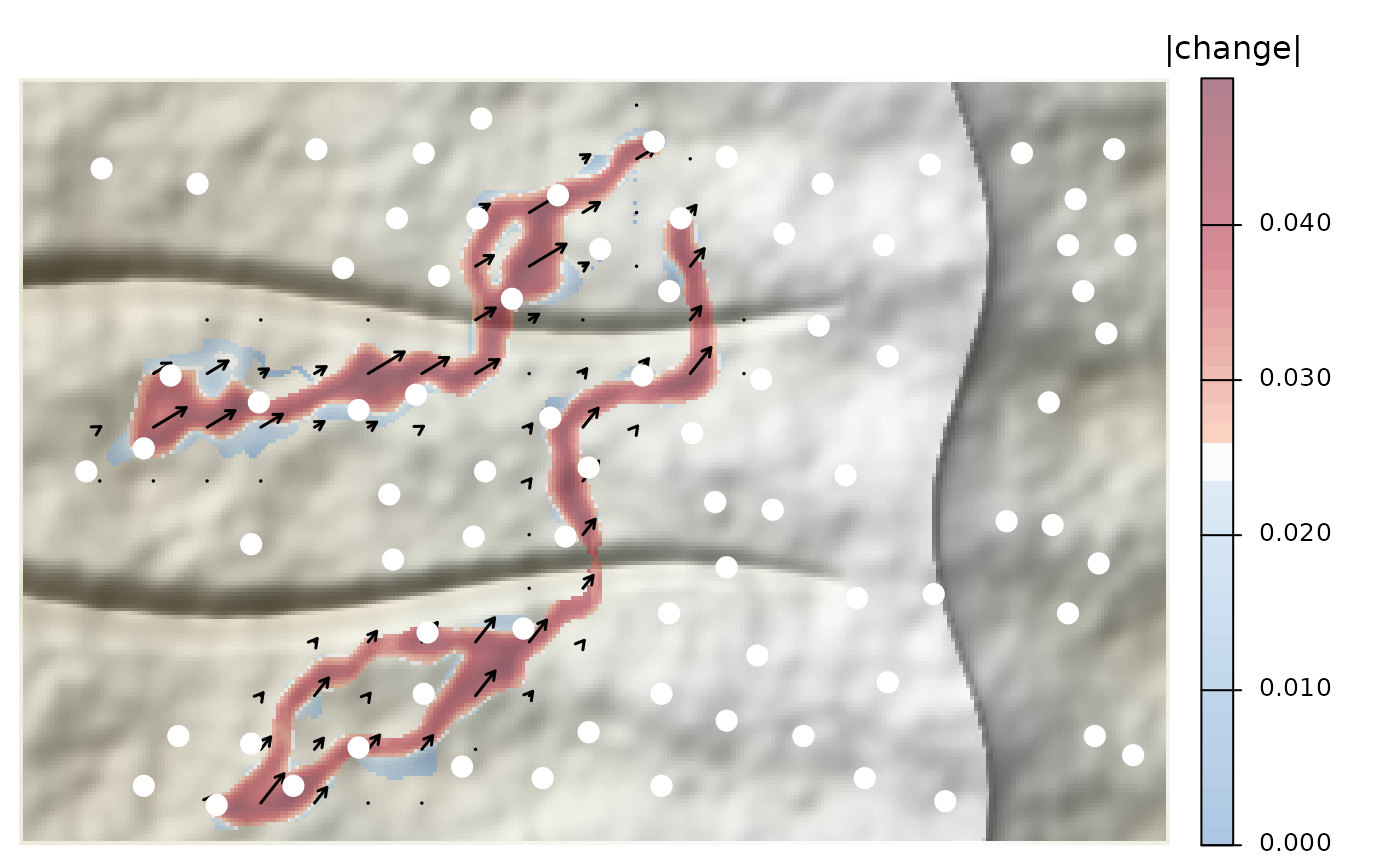
Draws a map from map_pairwise() over shaded relief. Change is colored on a three-tone scale: cool blue below threshold, a narrow white band at it, and red above it, so the areas under most pressure stand out. With a directional map, arrows from shift_arrows() show the net direction.

Usage

plot_shift(
  map,
  dem = NULL,
  sites = NULL,
  col_sites = "white",
  threshold = NULL,
  smooth = 5,
  alpha = 0.5,
  arrows = "vx" %in% names(map),
  cells = 14,
  scale = c("linear", "sqrt"),
  main = "",
  legend_title = "|change|"
)

Arguments

map: A map from map_pairwise().
dem: Optional elevation SpatRaster for the relief.
sites: Optional sf points to draw on top.
col_sites: Fill colors for sites (recycled, or one per site).
threshold: Value drawn in white. Defaults to the median of the map.
smooth: Width (in cells) of a moving-average window applied to the displayed surface only; 1 for none.
alpha: Opacity of the change layer.
arrows: Draw arrows (needs a directional map).
cells, scale: Passed to shift_arrows().
main, legend_title: Title and legend title.

Value

The map, invisibly.

Examples

# \donttest{
ex <- corridor_example(acc = TRUE)
v <- both_directions(data.frame(from = c("M03", "M08"), to = c("M40", "M45"), value = 0.05))
v$value[3:4] <- -0.05
plot_shift(map_pairwise(v, ex$acc, ex$sites), dem = ex$dem, sites = ex$sites)

# }